整理自李宏毅教授 2020 机器学习课程

• Regression
• Example Application + Step 1: Model
• Basic Concept - Where does the error come from?
  • Estimator
  • Bias and Variance of Estimator
    • Variance
    • Bias
    • What to do with large bias?
  • What to do with large variance?
  • Model Selection
  • Cross Validation
    • N-fold Cross Validation

Regression

• Stock Market Forecast

$$ f(“股票数据”) = Dow\ Jones\ Industrial\ Average\ at\ tomorrow $$

• Self-driving Car

$$ f(“无人车的Sensor”) = 方向盘角度 $$

• Recommendation

$$ f(“使用者A\ \ 商品B”) = 购买可能性 $$

Example Application

• Estimating the Combat Power (CP) of a pokemon after evolution

  用$x$代表宝可梦，其中$x_{s}$代表宝可梦的名称，$x_{cp}$，$x_{w}$代表重量，$x_{h}$代表身高。

$$ f(“宝可梦的参数\rightarrow x”) = “CP\ after \ evolution \rightarrow y” $$

Step 1: Model

• A set of function 去描述一个Model:

  $$ y = b + w\cdot x_{cp} $$

  $w$ and $b$ are parameters (can be any value), eg:

  $$f_1:y=10.0+9.0\cdot x_{cp} \f_2:y=9.8 + 9.2\cdot x_{cp} \f_3:y=-0.8-1.2\cdot x_{cp} \……$$

  用以上去描述宝可梦的函数式:

  $$f(x)=”CP\ after\ evolution” \rightarrow y$$

  这叫做 Linear model，

  $$ y = b + \sum{w_ix_i} $$

  其中，$x_i$：An attribute of input x, 用来描述 feature，$w_i$：weight，$b$: bias 。

• Step 2: Goodness of Function

  引入一些数据来作为 $y=b+w\cdot x_{cp}$ 的 input，比如，第一个数据为杰尼龟的数据，用$x^1$来表示第一个数据的数据集，对应的 output ，即卡咪龟的数据集，用 $\hat{y}^1$ 代表。其他数据以此类推。

  接下来的 Training Data 假设就是 10 只宝可梦。即，

  $$(x^1, \hat{y}^1)\\ (x^2, \hat{y}^2)\… \(x^{10}，\hat{y}^{10})$$

  对应图像如下，

  

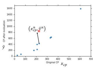
  图中任意一点的值为 $(x^n_{cp}, \hat{y}^n)$。

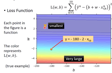
  在有了 training data 以后，需要定义另一个Loss function $L$: 其中input 为对应的 function，output 即为 how bad it is，即：

  $$L(f) = L(w, b)\\ =\sum^{10}{n=1}(\hat{y}^n - (b+w\cdot x^n{cp}))^2$$

  衡量参数的好坏, 即$w$ 和$b$ 的好坏，

  其中里面的括号中为 Estimated y based on input function，而 $\hat{y}^n$即为真实至，而$L(f)$则给出 Estimation error。

  $\sum$来 Sum over examples。

  图像为，

  

• Step: Best Function

  在建立了 A set of function 之后，要 pick the BEST Function，

  $$\begin{aligned}f^{}=& \arg \min _{f} L(f) \w^{}, b^{*} &=\arg \min {w, b} L(w, b) \&=\arg \min _{w, b} \sum{n=1}^{10}\left(\hat{y}^{n}-\left(b+w \cdot x_{c p}^{n}\right)\right)^{2}\end{aligned}$$

  可以利用 Gradient Descent 来解这个 function。

• Step 3: Gradient Descent，来解$w^{*}=\arg \min_{w}L(w)$

  • Consider loss function $L(w)$ with one parameter w:

    • 首先随机选一个起始值 $w^0$

    • Compute

      $$\left.\frac{dL}{dw}\right

      _{w=w^0}$$

      用图像来表示即为，

      

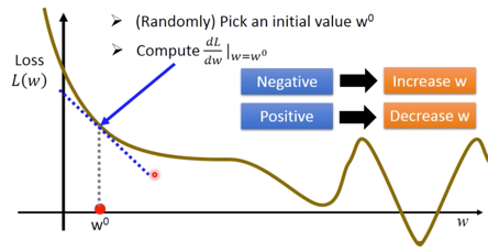
      寻找下一个$w^1$的值，即为

      $$w^1 \leftarrow w^0 - \left.\eta \frac{dL}{dw}\right

      _{w=w^0}$$

      其中 $\eta$ 被称为 “learning rate“，越大学习速度越快。

    • 下一步重复 Compute $$\left.\frac{dL}{dw}\right| _{w=w^1}$$

    • … Many iterations ( T times )

      这时候的情况如下图：

      

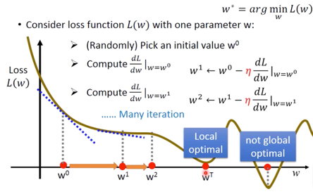
      这时获得了 Local optimal $\rightarrow w^T$，但注意是并非 Global optimal 。

  • 如果有两个参数呢?

    对应公式如下，

    $$w^, b^ = \arg \min_{w, b}L(w, b)$$

    • 随机 Pick an initial value $w^0, b^0$

    • Compute

    $$\left.\frac{\partial L}{\partial w}\right

    _{w=w^{0}, b=b^{0}},\left.\frac{\partial L}{\partial b}\right

    _{w=w^0, b=b^0}$$

    • 分别更新 $w$ 与 $b$ 的值

    $$ w^1 \leftarrow w^0 - \left.\eta\frac{\partial L}{\partial w}\right

    _{w=w^0, b=b^0}\ b^1 \leftarrow b^0 - \left.\eta\frac{\partial L}{\partial b}\right

    _{w=w^0, b=b^0}$$

    • Compute

    $$ \left.\frac{\partial L}{\partial w}\right

    _{w=w^1, b=b^1}, \left.\frac{\partial L}{\partial b}\right

    _{w=w^1, b=b^1}$$

    • 再次更新 $w$，$b$ 的值

    $$ w^2 \leftarrow w^1 - \left.\eta\frac{\partial L}{\partial w}\right

    _{w=w^1, b=b^1}\ b^2 \leftarrow b^1 - \left.\eta\frac{\partial L}{\partial b}\right

    _{w=w^1, b=b^1}$$

    • 反复重复这个步骤最终获得 loss 相对比较小的 $w$ 和 $b$ 的值

    • 而 $\nabla L$ 即为 gradient ：

    $$\nabla L=\left[\begin{array}{l}\frac{\partial L}{\partial w} \\ \frac{\partial L}{\partial b}\end{array}\right] _\text { gradient }$$

      其中，将两个偏微分排成一个 vector
    

    • 示意图如下，

    

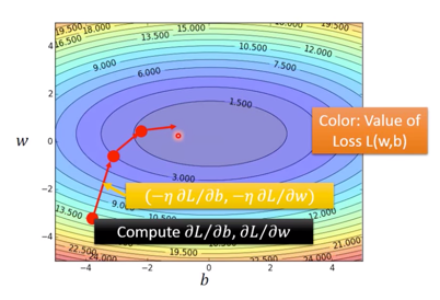
    其中每一次的 gradient 即为等高线的法线法向。

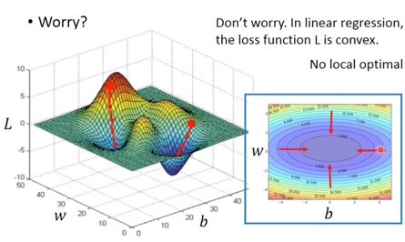
    • 但用这种方法，会出现问题，即如下图左侧所示，如果起点不同可能会找到不同的输出值，但实际上，利用这种方法是不会产生 local optimal 的

    

    • Formulation of $\partial L / \partial w$ and $\partial L / \partial b$，即为

    $$\begin{array}{l}L(w, b)=\sum_{n=1}^{10} ({\left.\hat{y}^{n}-\left(b+w \cdot x_{c p}^{n}\right)\right)^{2}} \\\frac{\partial L}{\partial w}=? \sum_{n=1}^{10} 2\left(\hat{y}^{n}-\left(b+w \cdot x_{c p}^{n}\right)\right)\left(-x_{c p}^{n}\right) \\\frac{\partial L}{\partial b}=? \sum_{n=1}^{10} 2\left(\hat{y}^{n}-\left(b+w \cdot x_{c p}^{n}\right)\right)(-1)\end{array}$$

  • How’s the results?

    

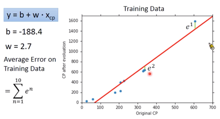
    Error 值即为真实值与预测值之间的距离。可以获得 Average Error on Training Data为，

    $$ \sum_{n=1}^{10}e^n = 31.9 $$

  • 但是真正关心的应该是 Generalization，What we reaaly care about is the error on new data (testing data)

    于是又取了十只 Pokemon，情况如下

    

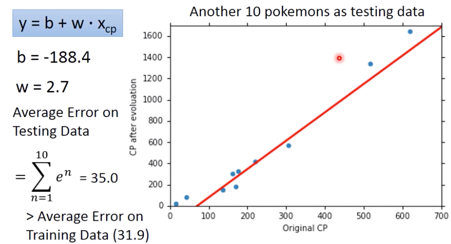
    而新的数据中的 Average Error on Training Data 为 35.0

  • How can we do better

    • 从上图中可见在CP较低和较高的区域，拟合不好，于是我们选择令 Selecting another Model

      $$ y = b+ w_1\cdot x_{cp}+w_2\cdot (x_{cp})^2$$

      找出 Best function，这时

      $$ b= -10.3, \w_1=1.0, w_2=2.7*10^{-3}\\ \text{Average Error} = 18.4$$

      

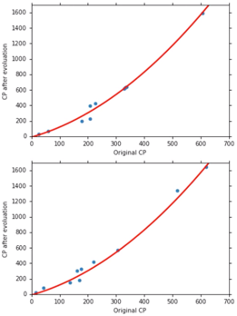
      重新取 10 只 Pokemon 得出，Average Error = 18.4

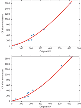
    • Better! Could it be even better?

      引入更复杂的model，

      $$ y = b + w_1 \cdot x_{cp}+w_2\cdot (x_{cp})^2 + w_3\cdot (x_{cp})^3$$

      找出 Best Function，

      $$ b=6.4, w_1=0.66\\ w_2=4.310^{-3},\\ w_3=-1.81-^{-6}, \Average Error = 15.3$$

      同样重新取 10 只 Pokemon ，得出 Average Error = 18.1

      

    • 用同样的方法，Try to make it better

      $$ y = b + w_1\cdot x_{cp}+ w_2\cdot (x_{cp})^2 + w_3\cdot (x_{cp})^3 + w_4\cdot (x_{cp})^4$$

      并获得图像，

      

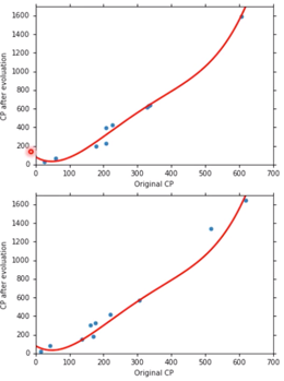
      这时的 Average Error = 14.9，但重新取 10 只 Average Error = 28.8 变得比之前更高了

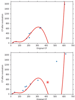
    • 继续使用更加复杂的 Model，结果会变得更加糟糕

      $$ y = b+w_1\cdot x_{cp} +w_2\cdot (x_{cp})^2 + w_3\cdot(x_{cp})^3 + w_4\cdot (x_{cp})^4 + w_5\cdot (x_{cp})^5 $$

      

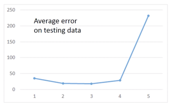
    • 分析这 5 个 Model，对这5次的 Training Data 的 Average Error 进行统计，如下图

      

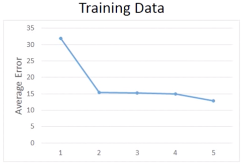
      这是因为更复杂的 Model 的 Function Space 会包含低级的 Model Space，如下图描述

      

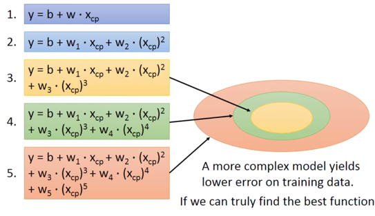
      但如果针对于，Testing Data，则情况会不同，

      

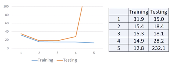
      A more complex model does not always lead to better performance on testing data, This is Overfitting.

      而当 Model 的复杂程度在第 4 次和第 5 次时，就发生了 Overfitting。

• What are the hiden factors?

  在计算CP值时，前面的 input 数据选用的只有杰尼龟一种，一旦要是，但是要去 make a more general model，就要考虑Pokemon的种类这一问题。

  

  如何解决这个问题呢？

  • Back to step 1: Redesign the fuction set of the Model

    可以套用 if 语句：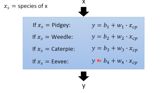

    

    接下来，我们需要将加入if语句的 Model 改写为 Linear model ($y=b+\sum{w_i x_i}$)：

    $$\begin{aligned}y=& b_{1} \cdot \delta\left(x_{s}=\text { Pidgey }\right) \&+w_{1} \cdot \delta\left(x_{s}=\text { Pidgey }\right) x_{c p} \&+b_{2} \cdot \delta\left(x_{s}=\text { Weedle }\right) \&+w_{2} \cdot \delta\left(x_{s}=\text { Weedle }\right) x_{c p} \&+b_{3} \cdot \delta\left(x_{s}=\text { Caterpie }\right) \&+w_{3} \cdot \delta\left(x_{s}=\text { caterpie }\right) x_{c p} \&+b_{4} \cdot \delta\left(x_{s}=\text { Eevee }\right) \&+w_{4} \cdot \delta\left(x_{s}=\text { Eevee }\right) x_{c p}\end{aligned}$$

    其中，

    $$ \delta(x_s = Pidgey) \ \ \left{\begin{array}{ll}=1 & \text { If } x_{s}=\text { Pidgey } \\ =0 & \text { otherwise }\end{array}\right.$$

    这样就有:

    $$ if \ x_s = Pidgey，\\ y = b_1 + w_1\cdot x_{cp} $$

    其中，

    $$\delta(x_s = Pidgey)$$

    这一项即为 Linear model 中的 $x_i$，也就是 feature

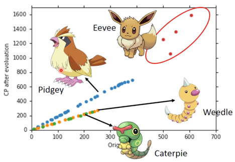
    引入不同 $x_s$ 后的分析图像如下图，

    

    从图中可见，不考虑伊布的曲线fit的不好，是因为伊布可以进化为不同的精灵，但其他宝可梦也有一些或多或少fit不好的情况，可能是进化时候加了一个 random number，但也可能不是 random number，也可能有其他factors

  • Are there any other hidden factors？

    

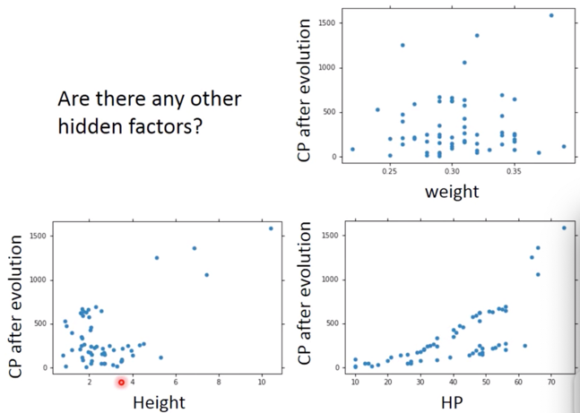
    对待这个问题，有可能是很多因素导致的，如 weight，HP 等等，那么如何解决这个问题呢？我们可以将所有的能考虑到因素加进去：

    

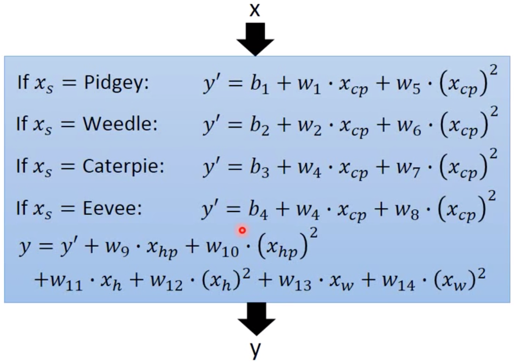
    这么复杂的 Model 给出了很低的 Training Error = 1.9，但Testing Error 却非常糟糕 = 102.3，发生了严重的 Overfitting。

    解决这个问题，我们要引出下一个概念：

  • Back to step 2: Regularization，重新定义我们的 Loss Function，将不好的去掉

    即在原有的 Loss function 后添加一项：

    $$ L = \sum_n(\hat{y}^n - (b + \sum{w_i x_i}))^2 + \lambda \sum(w_i)^2$$

    而这个 $\lambda\sum(w_i)^2$ 项，The functions with smaller w_i are better

    Why smooth functions are preferred?

    比如我们在 input $x_i$ 的基础上，增加为 $x_i + \Delta x_i$，则此时 对于 $y=b+\sum w_i x_i$ output 变为 $w_i\Delta x_i$，则当 $w_i$越小，input 对 output 影响越小，这样 function 也就会比较平滑

    If some noises corrupt input $x_i$ when testing，也就是是说 function 如果变得不平滑了，A smoother function has less influence。

    

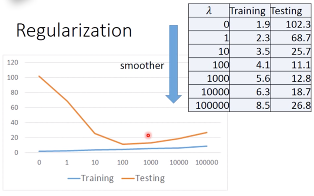
    首先可以确定，当 $lambda$ 越大，function 越平滑，但 function 越平滑，Traning data error 越大，这是因为：Larger $lambda$，considering the training error less，越倾向于考虑 $w_i$ 本来的值。

    但 Testing error 却发生不同的变化，可见：We prefer smooth function, but don’t be too smooth。

    所以我们需要调整一个较好的 $\lambda$，这是非常重要的。

  • 另外需要注意的是，对于 Regularization 项：

    $$\lambda\sum(w_i)^2$$

    只包含有 $w_i$，但却没有 $b$，其实在考虑 Regularization时，不需要考虑 bias。因为加 bias 只会对 function 进行平移，不会影响 function 的平滑度。

• Conclusion:

  • Gradient descent

    • Following lectures: theory and tips

  • Overfitting and Regularization

    • Following lectures: more theory behind these

  • We finally get average error = 11.1 on the testing data

    • How about another set of new data? Underestimate? Overestimate?

    • Following lectures: validation 来解决上面的问题。

Basic Concept - Where does the error come from?

在之前的实例中，我们发现选择不同的 Function Set，也就是选择不同的 Model，往往会给出不同的 Average error，而且越复杂的 Model，不见得会给出越低的 Error。

而其中 error 有两个来源：

1. 来自于 “bias”
2. 以及 “variance”

Estimator

对于一个 Estimator, 如

$$\hat{y} = \hat{f}(\text{Pokemon CP})$$

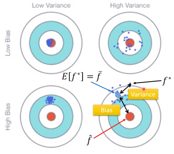
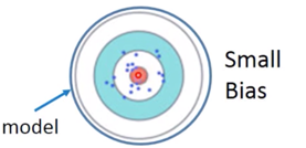
From this training data, we find $f^*$ ，那么有 $f^*$ is an estimator of $\hat{f}$。二者关系可以用下图表示，

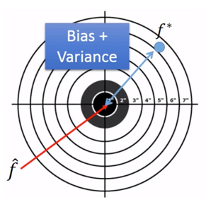
靶标的中心点是 $\hat{f}$，而 $f^*$ 则在偏离靶中心的位置，而这个偏离，就是又 Bias 以及 Variance 共同决定的。

Bias and Variance of Estimator

• Estimate the mean of a variable x

  • assume the mean of x is $\mu$
  • assume the variance of x is $\sigma^2$

• Estimator of mean $\mu$

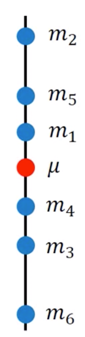
  • Sample N points: ${x^1, x^2, …, x^N}$

    $$ m = \frac{1}{N}\sum_n{n^n} \neq \mu$$

    这时 $m$ 和 $\mu$ 的值是不相等的，示意图如下

  

  • 但是如果我们计算这些 $m$ 的期望值，就会得到我们想要的 $\mu$

    $$E[m] = E\biggl[\frac{1}{N}\sum_n x^n\biggr] = \frac{1}{N}\sum_n E[x^n] = \mu$$

    这个问题就像打靶，每次打靶都会偏离中心，但当打靶次数足够多，最终这些偏离中心的打点的中心就是最终的期望。

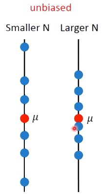
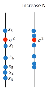
  • 这个散布在期望周围, 散的有多开取决于 $m$ 的 Variance ，这个 Variance 的表达式为，

    $$Var[m] = \frac{\sigma^2}{N}$$

    Varicance depends on the number of samples，如图所示

    

• Estimator of variance $\sigma^2$

  • Sample N points: {$x^1, x^2, …, x^N$}

    1. 首先估计 $m$ 的值，

       $$ m = \frac{1}{N}\sum_n x^n $$

    2. 之后再计算估计 $s^2$，

       $$ s^2 = \frac{1}{N}\sum_n (x^n - m)^2 $$

       这个 $s^2$ 可以用来估计 $\sigma^2$

    但是，需要注意，这个对于 $\sigma ^2$ 的估计是Biased estimator，

    $$ E[s^2] = \frac{N-1}{N} \sigma ^2$$

    也就是说 $s^2$ 的期望值并不正好等于 $\sigma^2$ ，如果我们增加样本量，这一现象就会减轻：

    

    用打靶来描述这件事情，如下图

• Parallel Universes

  

  而打靶打的准或不准是由 Variance 和 Bias 两部分共同决定的。

Variance

In all the universes, we are collecting (catching) 10 Pokemons as training data to find $f^*$

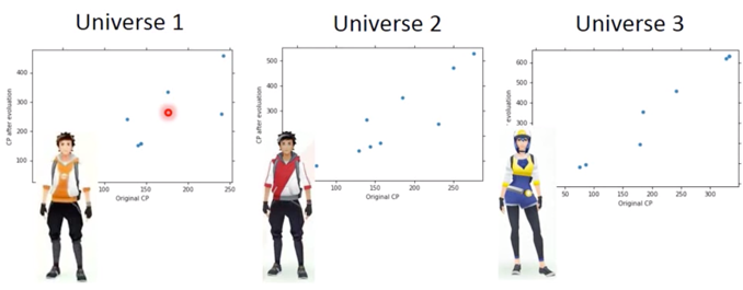
我们在不同宇宙中抓到的宝可梦是不一样的。

In different universes, we use the same model, but obtain different $f^*$

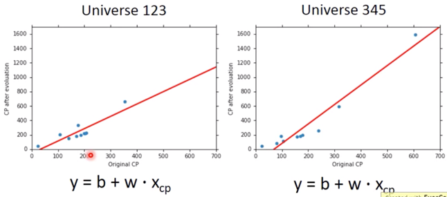
最终的结果如果我们用越来越复杂的 model ，就会给出越来越崩溃的结果,

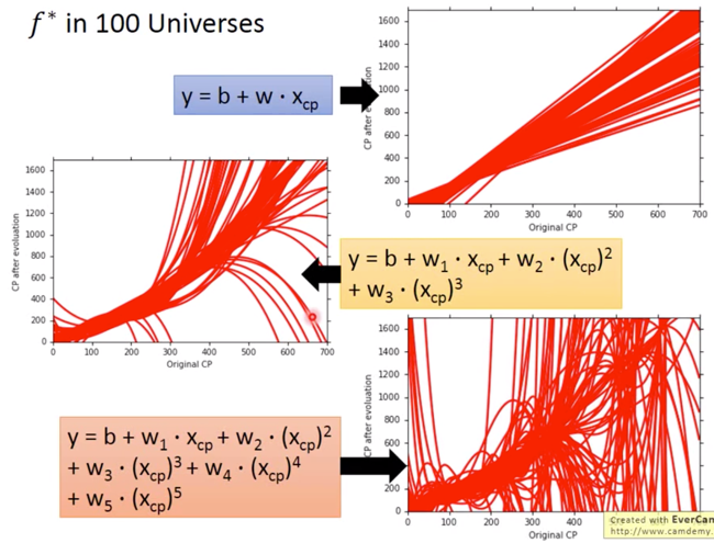
而这几种越来越复杂的 model 所带来的混乱的情况，用打靶来形容，如下图所示，

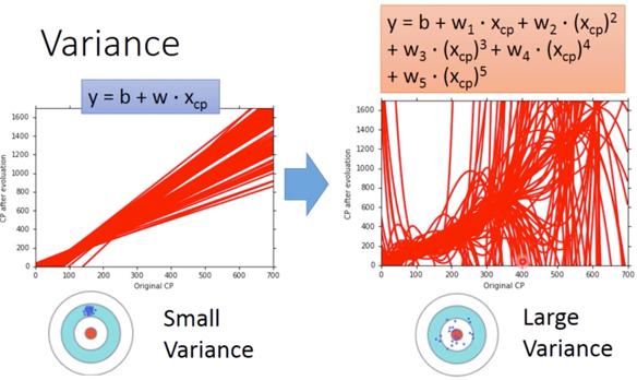
可以看出，越简单的 model，对应的 Variance 越小，这可以认为是因为，Simpler model is less influenced by the sampled data 。可以考虑一个极端的例子：

$$ f(x) = c $$

对于这个常值函数的 model，其 Variance = 0，不会受到 sampled data 影响。

Bias

$$ E[f^*] = \overline{f}$$

• Bias: If we average all the $f^*$, is it close to $\hat{f}$

  • 先引入打靶问题，来描述 Bias 大小对于靶标的影响，

    

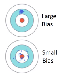
    可见，如果 Bias 很小，即使数据很离散，其平均值 $\overline{f}$ 也会很接近 $\hat{f}$。

  • 下面需要确定一条 $\hat{y}$，我们只能先假设一个 $\hat{f}$

    

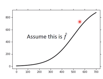
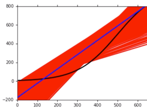
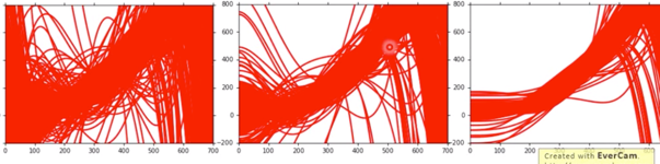
  • 然后我们分别对不同复杂程度下的 model 给出的 $\overline{f}$ 与 $\hat{f}$ 之间的关系，如下图

    

    • 上图是描述一次的 Model，图中曲线标注情况如下：

      Black curve: the true function $\hat{f}$

      Red curves: 5000 $f^*$

      Blue curve: the average of 5000 $f^* = \overline{f}$

    • 当考虑一个较为复杂的三次 Model，如下图

      

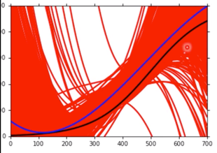
      虽然单独每一次和 $\hat{f}$ 可能相差很多，但平均下来与 $\hat{f}$ 却较为接近。

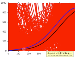
    • 当复杂程度继续升高，即考虑五次的 Model，$\overline{f}$ 则进一步趋近于 $\hat{f}$，如下图所示:

      

对于以上现象，可以从 function space 的角度来解释，即如果 Model 没有那么复杂，它对应的 function space 就相对较小，可能并没有包含 Target，如下图，

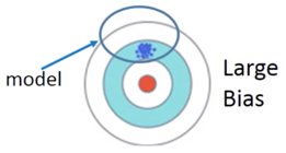
相反如果 Model 比较复杂，对应上述 5 次的 Model，其 function space 较大，就可能包含了 Target，如下图，

What to do with large bias?

综合起来，存在两种 error，即：

1. Error from bias
2. Error from variance

这两种对应的 Error 的关系如下图，

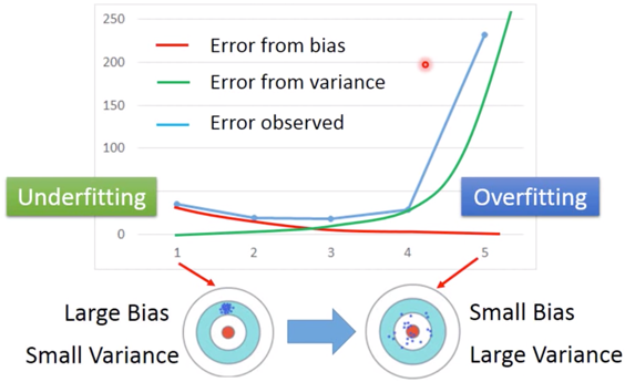
而由于 bias 引起 Error，我们称之为 Underfitting ；由于 variance 引起的 Error，我们称之为 Overfitting。

• Diagnosis:

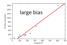
  • If your model cannot even fit the training examples, then you have large bias: Underfitting

    

  • If you can fit the training data, but large error on testing data, then you probably have large variance: Overfitting

• For bias, redesign your model:

  • Add more features as input

  • A more complex model

What to do with large variance?

• more data

  

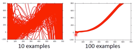
  It’s very effective, but not always practical. 也可以根据经验给一个经验的 Model

• Regularization

  通过 Regularization，使得曲线更加平滑，如下图所示：

  

  但是这样做，会伤害到 bias

Model Selection

• There is usually a trade-off between bias and variance.

• Select a model that balances two kinds of error to minimize total error

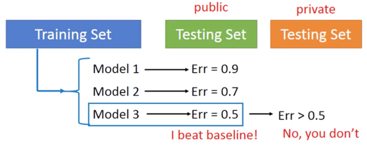
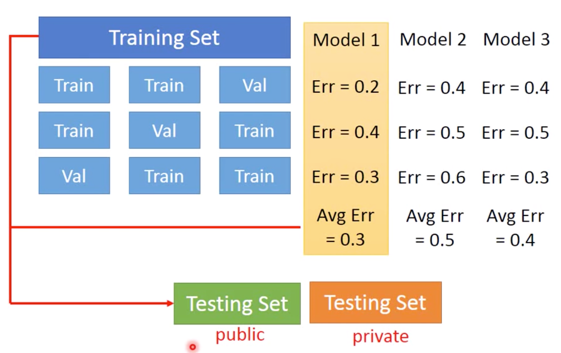
• What you should NOT do:

  

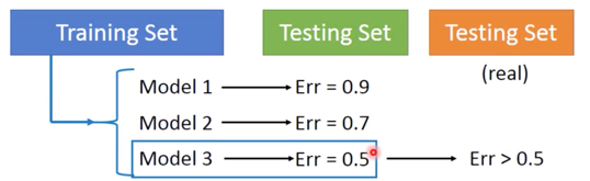
  注意不要直接选择 Model 3，因为绿色的 Testing Set 本身有着自己的 bias，而与实际上的 橙色的 Testing Set 不同 ( $Err > 0.5$ )。

  为了更好的理解这个问题，给出下面的举例：Homework 中的情况

  

  更好地理解，比如说小明在班级里排名第一，但在全校可能排不上名次。

  那么如何解决这个问题呢？

Cross Validation

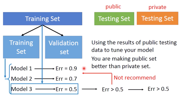
1. 可以将 Training Set，分成两部分，即 Training Set 和 Validation Set
2. 再通过新的 Training Set 计算出 Error 以后，选出最佳的 Model
3. 再将全部 Training Set 加进去，计算public Tesing Set 的 Error，这时的 Error 会比之前的 Error 更大，但更加接近真实的 private Testing Set。
4. 但不建议在知道 pulic Error 很大以后，再返回去修改前面的 Model，因为这样会引入这次 Public Testing Set 中的 bias。

• Using the results of public testing data to tune your model

• You are making public set better than private set，在 public 看到的 performance 没办法反应在 private 上的 performance了

如果将 Training Set 分开 Validation Set 时，发现 Validation 的 bias 也有问题怎么处理呢？

N-fold Cross Validation

如果你不相信某一次 Training 结果，可以按下图方式进行：

利用这种方法，根据三次实验后的 Average Error，再去进行比较。原则上，少去根据 Testing Set 调整 Model 的话，往往最终得到的 Testing Set 会比较小。